5 Really Useful Excel Tricks & Tips

5 Really Useful Excel Tricks & Tips

These really useful Excel tricks and tips can increase your productivity and save you time.

1 – Repetitive Operations

Repeat Last Action F4 or Ctrl + Y

Life is full of repetition and most of the time not only is that boring but we are not always consistent. Using function key F4 (When the mode indicator = READY) will repeat the last action with most operations in Excel. You can go on to use it indefinitely.

So if that row you just inserted that wasn’t enough – press F4
That complex cell formatting in the Format Cells dialog box that you need to repeat – press F4

Note: This also works in most Office applications. This is particularly useful when applying styles in MS Word.

Format painter

Whilst the “Repeat Last Action” feature is OK if you have just performed the action, worthy of mention is the Format Painter. Just in case you missed this one, double clicking the format painter button will give you infinite Paste Formats until you turn it off.

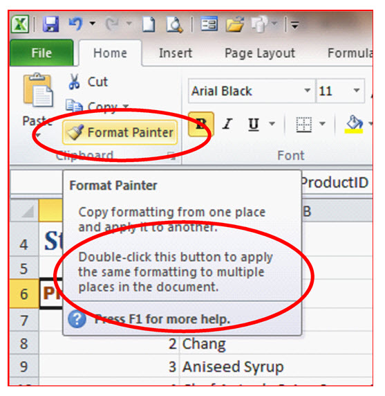
To turn it off either use the Escape key or press the Format Painter button again.

2 – Accurate and Quick Data Selection

When working with large data sets, quickly selecting the cells containing the data can be accomplished with a couple of shortcut key combinations.

Go to the End of a Data Block

The Ctrl key can be used with the keyboard arrow keys and Excel will ‘Go’ in the direction of the arrow to the end of the data block. This might be the start of the data block or the end of the data block. Note that any gaps in the data may catch you out. It works best with contiguous data.

Ctrl + Arrow > Select (Go to) the end of the data block
Extend (or Contract) a Selection

In any Windows application you can extend a selection by holding the SHIFT key whilst you use any navigational technique to redefine the selection. This includes clicking the mouse or keyboard shortcuts.

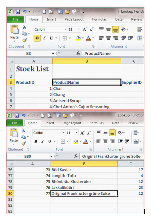
So with cell B3 selected in the example and Ctrl + Down Arrow pressed (Once) then Excel scrolls down and selects the last populated cell in the block of data, stopping at the cell next to the empty cell.

That’s Cell B80 in the example.

Do this a second time and you will find yourself on the last row if there is no more data in that column. That’s row 1,048,576 unless you are still in compatibility mode (65,536).

Combine Extend a Selection with Go to the End of a Data Block

Select the cell at one “End” of the range that you intended to select.

Hold the Shift key down
Press Ctrl + Arrow
Release the Shift key

Your block of cells is now selected. You can continue this technique to extend the range further. If you need to make minor adjustments then then just use:

Shift + Arrow

3 – Are you Protected?

So you have built this amazing Excel Workbook which you expect your fellow employees to be using for the next decade. It’s really clever but you’re concerned that users might
damage it. Not a problem because you have discovered Worksheet Protection. Just in case you haven’t:

Protecting a Worksheet
Unlocking Cells

By default all cells are “Locked”. The effect of this, however, is only applicable when the Worksheet is “Protected”.

Select the cells that you intend users to be able to edit and invoke “Format Cells”:

On the Protection Tab:

Note that the default for the Locked Check box is: Selected Uncheck the Locked check box to enable User Editing.

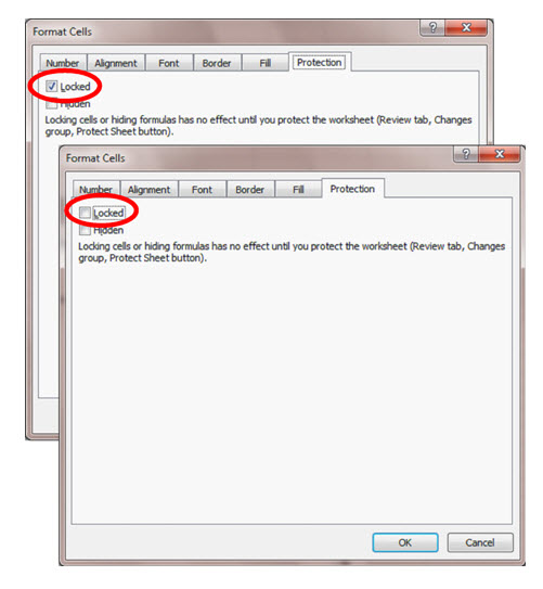
Tip: You might consider a suitable fill colour to indicate which cells are unlocked.
Tip: If you are working on a used workbook it might be a good idea to select the entire sheet and force all cells to be locked if you have any doubts about the cell status.
“Switching On” Protection

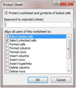
When you have finished developing your workbook and you are ready to ‘publish’ you will need to remember to “Switch On” Sheet Protection:
Review Tab > Changes Group > Protect Sheet:

The password is optional.

Caution: Allowing users to perform any of the unchecked options in the illustration rather defeats the point of the operation.

Note: This needs to be repeated for each sheet in the workbook that you wish to protect. Protecting a Workbook does NOT do this.(It stops users moving sheets within the workbook etc.)

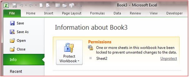
So is your Worksheet Protected?

There is no visible indicator that sheet protection is on or off. (Unless you happen to be on the Review tab and note the status of the Sheet Protection button).

There is no indication as to which cells are unlocked unless you applied some formatting.

Even using Lotus 1-2-3 on a black and white monitor in the 80s you could tell which cells were unlocked as the contents showed bright and the word PROT appeared in the status bar. (It is probably about time Microsoft sorted this one out. Knowledge base: Q161245 is not really good enough).

But at least in Excel 2010 you can obtain a summary:

The Trick

In Excel the use of the TAB key normally works as follows:
With just one cell selected:
Tab will select the next cell to the right. (Shift & Tab will select the next cell to the left.)

With multiple cells selected:
Tab will select the next cell to the right within the selection (Shift & Tab will select the next cell to the leftwithin the selection.)

However with Sheet Protection ON the TAB key works as follows:

With just one cell selected:
Tab will select the next UNLOCKED cell.

With multiple cells selected:
Tab will select the next UNLOCKED cell within the selection.

Perform an Audit of Unlocked Cells.
Start in cell A1 of your protected sheet and just keep pressing TAB to visit every UNLOCKED cell. If you find yourself going outside the Active Area / UsedRange then it is probable that sheet protection is not ON.

4 – Tidy Files – Controlling the Active Area / UsedRange

I frequently receive Excel files whose size is much larger than I would expect. Also, in the process of getting my head around what the author has been doing in each sheet I always check the location of the Active Area or UsedRange:

Ctrl + End Go to the end of the Active Area / Used Range

This is often much further beyond what you might expect. Caused by accidents, inappropriate formatting of cells etc.

By tidying up the Active Area / Used Range the file size is often significantly reduced and in any event we can be confident as to where each sheet “ends”.

Suggested procedure to tidy up a Worksheet’s Active Area

• Backup the file.
• Identify where you think the bottom right hand corner of the workbook should be.
• Check all columns to the right to ensure no significant data is located here. (Ctrl + up / down arrow is useful here. See Go to the End of a Data Block elsewhere in this article.)
• Check all rows below to ensure no significant data is located here. (Ctrl + left / right arrow is useful here. See Go to the End of a Data Block elsewhere in this article.)
• Select all ‘unnecessary’ columns and delete them.
• Select all ‘unnecessary’ rows and delete them.
• Save the file. This forces Excel to re-evaluate the “UsedRange”.
• Test with Ctrl + End
• Out of interest compare the file sizes before & after.

5 – Create a Custom List for Use with AutoFill or Custom Sort

Have you have used an AutoText entry in Word and wondered if Excel had an equivalent? This trick came to light when dealing with a customer whose organisation had many divisions and these were frequently required to be listed in Excel.

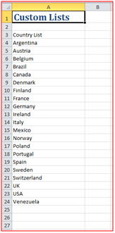
Create a Custom List by Example

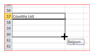
Create a vertical list of the items you require in your Custom list. Ensure that they are headed by a short memorable description. Sort the list into your preferred sequence.
Select the list including the header. (“Country List” in the illustration).

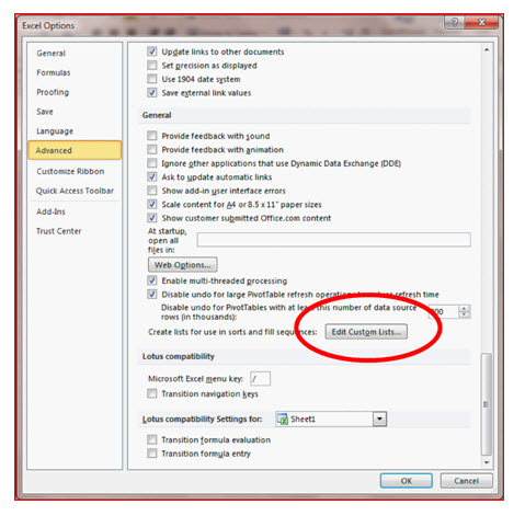
In Excel 2010 and above:
File > Options > Advanced > Scroll right down to the bottom >

Edit Custom Lists…

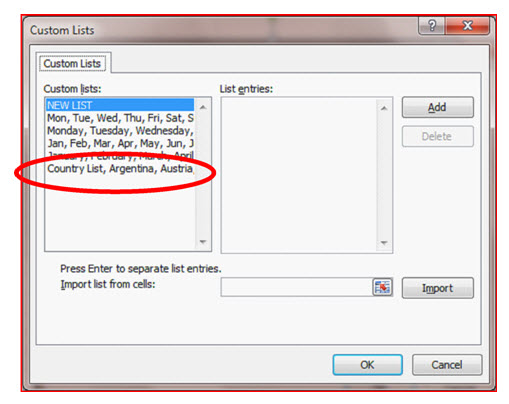
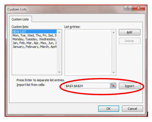
You are now able to import the list into your Custom Lists as follows:
Press Import

Note:
Your custom list is now saved in your registry and will be available to you in any workbook open on your computer. In Excel 2010 it is located in:
[HKEY_CURRENT_USER\Software\Microsoft\Office\14.0\Excel\Options]
and is saved when Excel is closed.

It is only saved in the file if the custom list is used to sort data.

However, if you open the workbook on another computer or server, you do not see the custom list that is stored in the workbook file in the Custom Lists dialog box that is available from Excel Options, only from the Order column of the Sort dialog box. The custom list that is stored in the workbook file is also not immediately available for the Fill command.

If you want, you can add the custom list that is stored in the workbook file to the registry of the other computer or server and make it available from the Custom Lists dialog box in Excel Options. From the Sort dialog box, under the Order column, select Custom Lists to display the Custom Lists dialog box, select the custom list, and then click Add.

To use your custom list with Autofill
Enter your short memorable description.
With the cell selected, place the mouse over the fill handle and drag down.

Watch the auto tip to monitor when to stop. The list will just repeat if you go too far.