Our expert trainers can help you get the best results.
If you would like any further information please contact one of our training advisors.

This article contains 5 extra Excel Tricks Tips and more sage advice on using Microsoft Excel.
During our training courses it is very apparent that Delegates all have their preferred methods of driving their computer and I find it interesting just how committed Delegates are to their particular method. I am very impressed with those who have taken to learning keyboard shortcuts and use them without even giving them a second thought.
However, I thought I would just review your options and you can decide for yourself how you might not only improve your speed but also your accuracy whilst remaining comfortable with your method mix.
The ribbon/ menu
Pros
Useful for a structured approach to driving your application.
Can be customised In Office 2010 and above.
Cons
Requires a few clicks.
Some choices are not where you might expect to find them. (Try finding Save Chart Template in Excel 2013. It’s not there! Use a right click.)
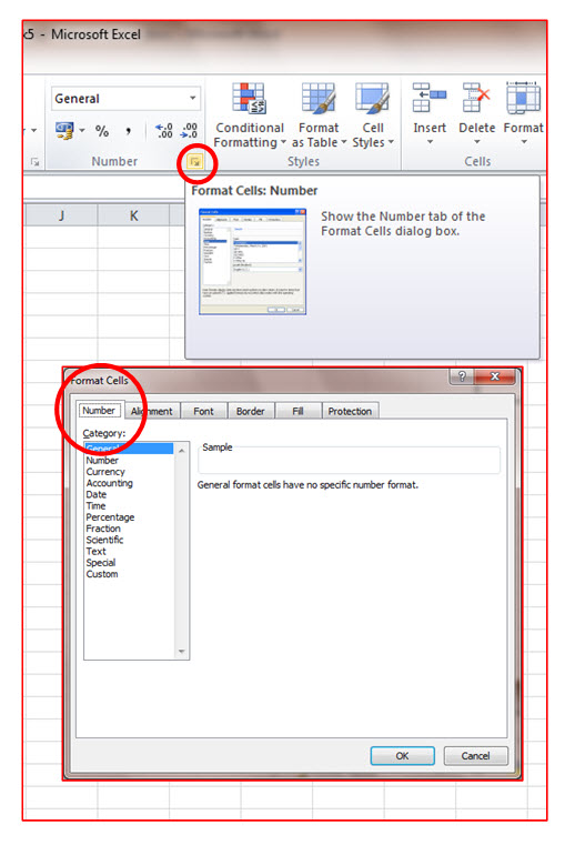
Tip
Look for Dialog Box launchers to quickly get to the “Fully Featured” dialog boxes.
The Right Click – The Context Menu
Pros
A great frustration reliever. Ensure that the point of the mouse is precisely over the object on which you wish to perform an operation. The context menus are getting better at each version.
They are often accompanied by a Mini toolbar.
Particularly useful in Charts where there so many discrete objects each with many properties.
Cons
Doesn’t always contain everything you might expect.
Tip
Take time to look at the choices available.
Keyboard Shortcuts
Pros
Used correctly, they are both predictable and quick.
Reduce repetitive strain injury issues.
Cons
Confusing when the wrong keys are pressed and an unexpected shortcut is invoked.
Tip
Those that work in all applications are well worth learning.
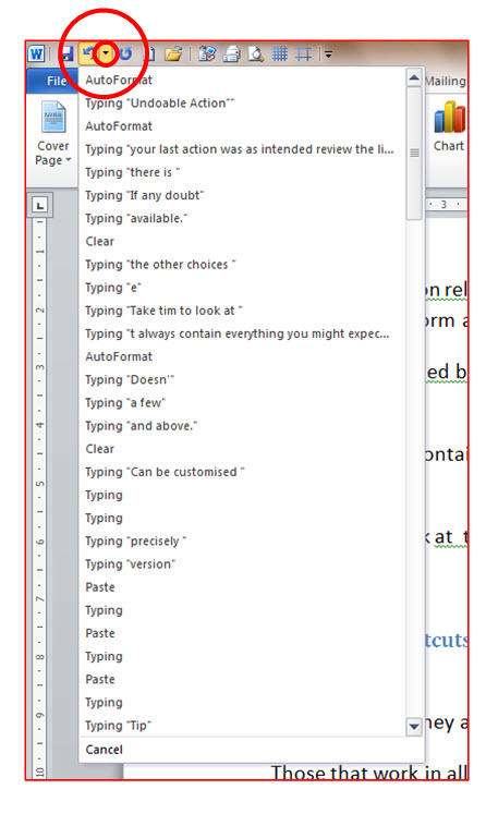
If there is any doubtthat your last action was as intended then review the list of “Undo-able Actions” from the drop arrow on the right hand side of the Quick Access toolbar’s Undo button.
Ctrl + Z is a shortcut for Undo (But you knew that!).
Warnings
The undo buffer in Excel is a common buffer for all workbooks that you are working on whereas in Word each document has its own undo buffer.
Since Office 2010 the Undo buffers are completely deleted after certain operations. For example delete a sheet and that’s all your undos deleted!
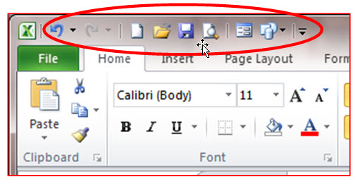
Quick Access Toolbar (QAT)
Pros
It is always available.
It can contain options which are not listed in the Ribbon.
Cons
With many items on the QAT it rather defeats the point.
Tip
With Office 2010 onwards you can export / import your QAT.
Right click on your favourite ribbon items to “Add to Quick Access Toolbar”.
To avoid interference with the Title Bar and file name choose “Show Below the Ribbon”.
Take the effort to customise it and use separators to create your own groups.
Warnings
Buttons on the QAT used to run a macro will have the full pathname of the file containing the macro embedded into the button definition. If the file containing the macro is renamed or moved then the button will need to be recreated otherwise it will attempt to run the macro in the original file. However, works well with your Personal.xlsb Workbook.
The Alt Key
The Alt key to left of the space bar will provide a method of driving the menus or ribbons in all Windows compliant programs. In older style (Pre Ribbon) menus the user can continue to work the menu by typing the underlined letter in the menu choice that they wish to make.
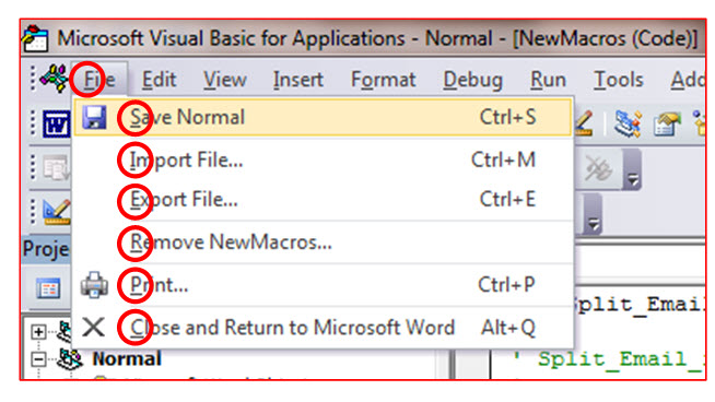
In this ‘Menu’ example:
The Alt key was pressed and then the letter F (For file.)
At this point the user could type:
S for Save
I for Import
E for Export
R for Remove..
P for Print
C for Close..
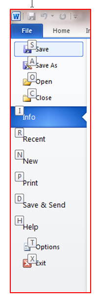
In this ‘Ribbon’ example:
The Alt key was pressed and then the letter F (For file.)
At this point the user could type:
S for Save
A for Save As
O for Open
I for Info
etc. as indicated by the tags.
Pros
If your keyboard skills are accurate you can be prompted through these keypresses to the point where you will start to remember them.
Cons
This will require more key presses than any specific shortcut. For Example in MS Word / Excel to format in bold:
Keyboard shortcut: Ctrl + B
Ribbon shortcut: Alt,H, 1
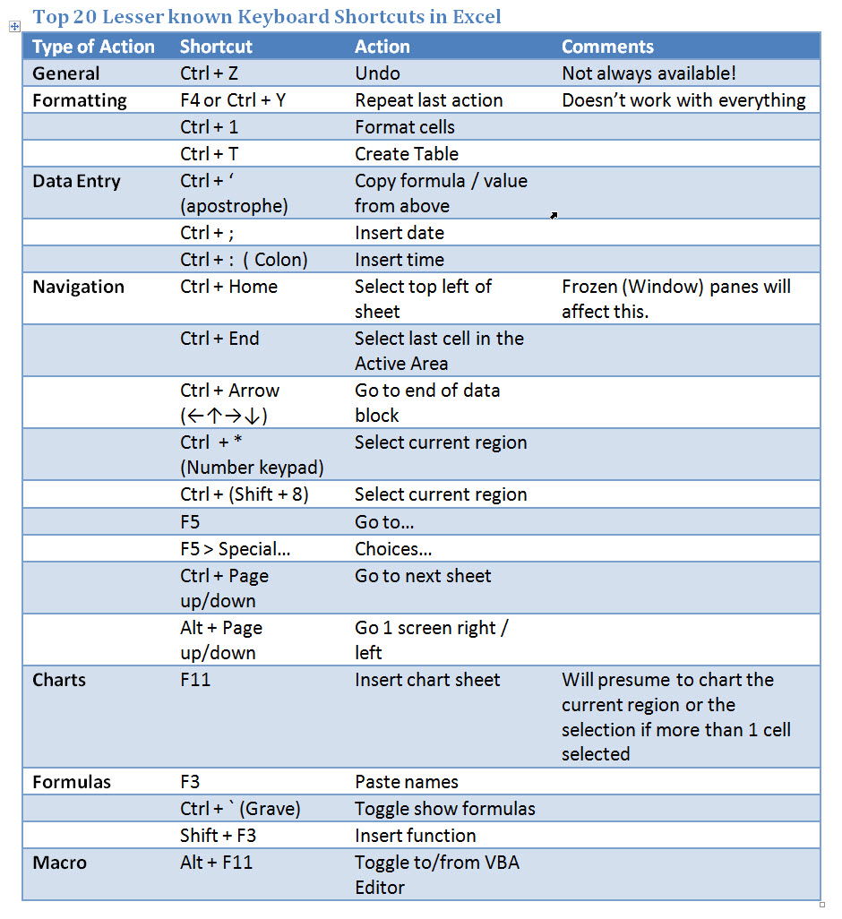
Conclusion – Useful Shortcut keys
There are over 160 shortcut keys available in Excel ranging from function keys to combinations of keys involving Shift + Key, Ctrl + Key, Alt + Key, Shift + Ctrl + Key.
Here are some of my favourites:
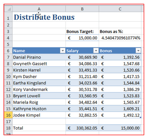
So you have €15,000 which you wish to use to reward your staff for their hard work. You want to be absolutely fair. It is to be a percentage of their salary. You try 5% and that’s too much:
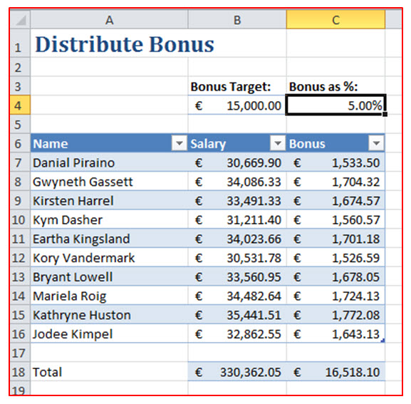
Let Excel work it out for you with a precision and speed that you will never achieve.
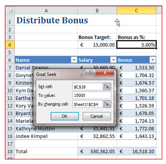
Goal Seeker
Goal seeker will try many values in one cell to attempt to obtain the result in a dependant cell that matches your requirement.
Data Tab > Data Tools Group > What-If Analysis > Goal Seek…
Note: The target “To value” cannot be a cell reference.
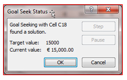
Closer Inspection of the result shows:
4.54047309610774%
That’s the maximum precision that Excel works to (15 digits).
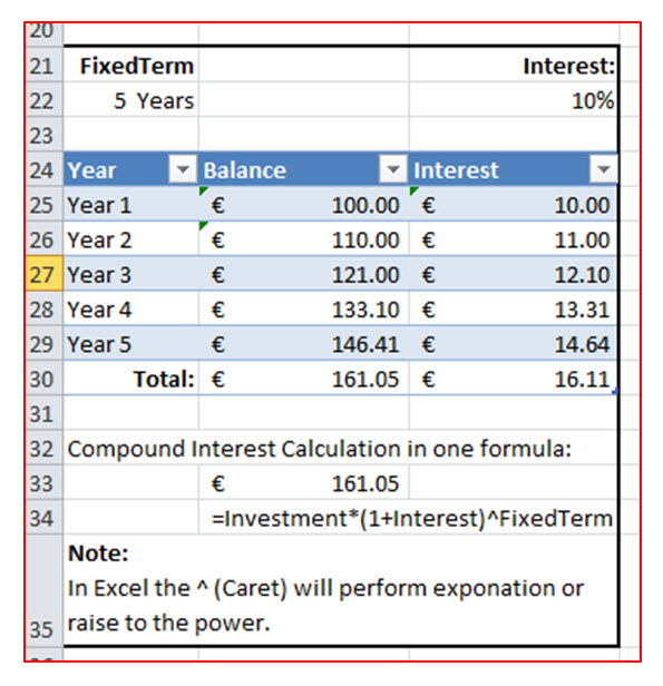
Another Scenario – Compound Interest:
Your savings are receiving compound interest of 10% per annum. (Not currently likely but a nice round number). They are invested for 5 years.
You could calculate interest for each year or, as shown in row 33 & 34, for the entire period.
Use Goal Seeker to work backwards from actual Interest received to deduce just what % interest rate you actually received.
Continuing the theme of true fairness in the workplace, imagine that you have been asked to place staff in random groups.
The following illustration shows a couple of functions and how to force recalculation of “Volatile Excel Functions”.
Column B uses the Excel Rand() Function which generates a random number between 0 and 1:
Cell B2=RAND()
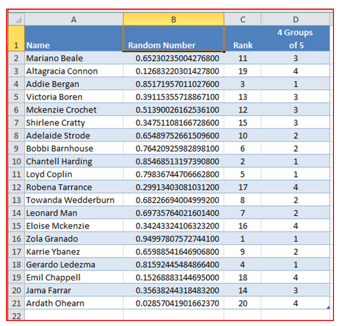
Column C Ranks the random number in relation to all the other random numbers in the range of interest. This will give a whole number in the range 1 to however many numbers are in the list:
Cell C2 =RANK.EQ(B2,$B$2:$B$21)
Column D is just a method of then grouping the results into the appropriate groups using the INT() function. We are looking for 4 groups of 5 staff members each. The INT() function rounds a number down to the nearest integer.
Cell D2 =INT((C2-1)/5)+1
If you don’t like the results use F9 to force Excel to recalculate all volatile functions like:
=Rand(), =Today(), =Now(), =Offset(), =Indirect(), =Info() & =Cell()
This is more of a warning than a tip.
Prior to the days of multi-threading multi-processor computers many of those of an Accounting persuasion noted that their large workbooks took so long to calculate that their keyboards either failed to respond or buffered their keystrokes whilst Excel was busy recalculating their workbook. The practice was to turn off Automatic Calculation:
Formulas Tab > Calculation Group > Calculation Options > Manual
You have to remember to manually force a recalculation.
Typically you would use F9.
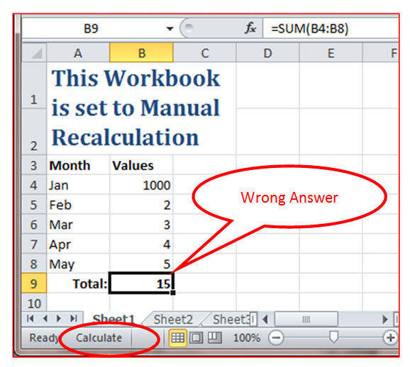
I have seen many examples where users have failed to note that their Workbook is in need of a recalculation. The clue is in the status bar and the word:
Calculate!
The absence of the prompt is “Evidence” that the sheet is not in need of recalculation. (It has no “Dirty” cells).
Infectious Manual Calculation Settings
As soon as you go down this route you will discover that what you thought was a Workbook setting is “Infectious”!
A look at the Excel Options suggests that it is indeed a Workbook setting:
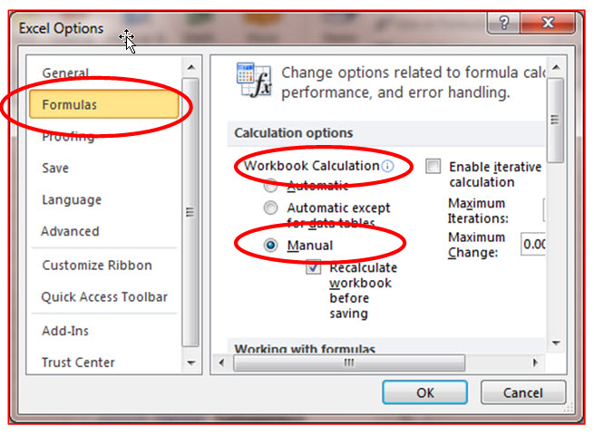
However, the Setting Migrates From File To File
The first file that you open in an instance of Excel will “Set” the rule for calculations for the Excel Instance. So if a “Manual Calculation Workbook” is open in Excel when you then open an “Automatically calculated workbook” the setting will “migrate” to the second file. If you then save that file, next time you open it you will discover that it has now become a “Manual Calculation Workbook”. The reverse is also true.
Tip
Avoid the problem. Don’t use Manual Calculation. Review you workbook, if you were to turn off Manual Calculation does it still make your Workbook unresponsive during recalculation?
If you must use a Manual Calculation Workbook investigate some simple macros to remind you to recalculate before Printing, before saving, on an open etc.
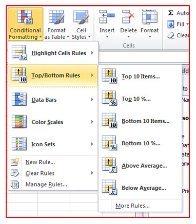
If you are looking to provide visual indicators in your lists, Tables and PivotTables take a detailed look into all the options available in Conditional Formatting:
Home Tab > Styles Group > Conditional Formatting >…
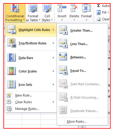
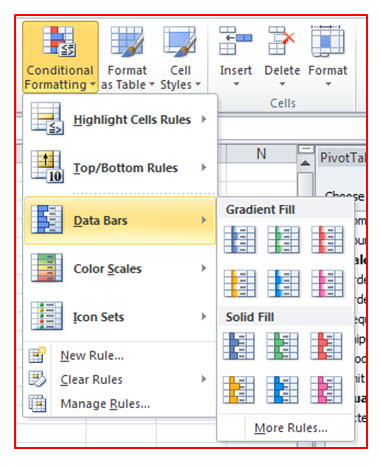
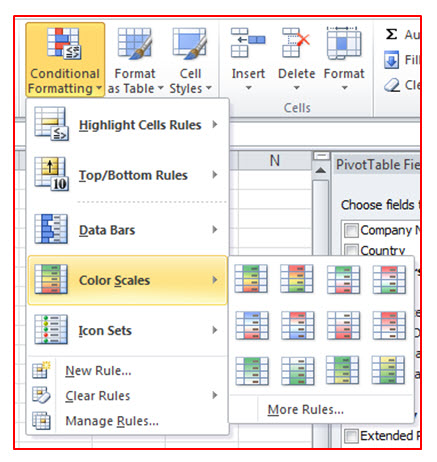
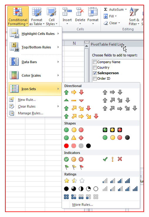
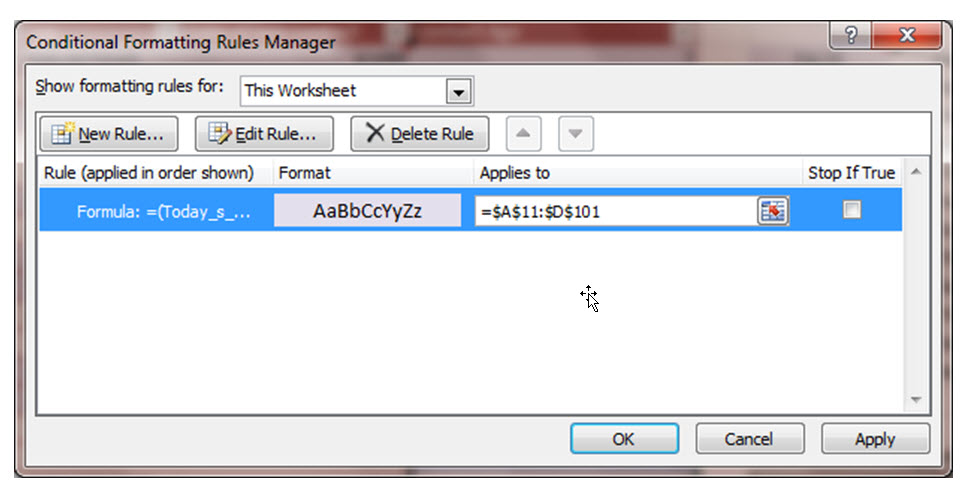
Use the Conditional Formatting Rules Manager to edit these defaults to suit your needs.
Highlight the entire row of interest
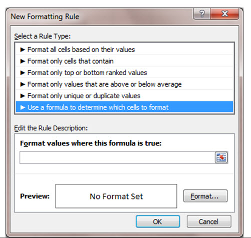
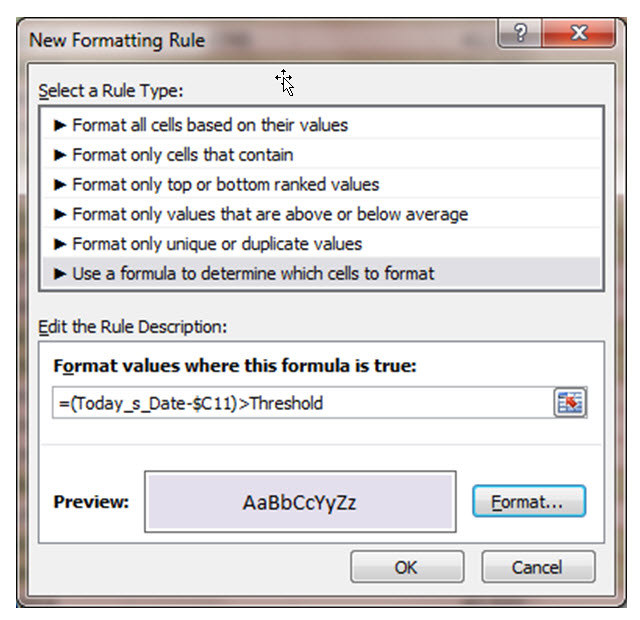
A frequently requested requirement is to flag up the complete row of data subject to some logic in a specific cell on that row. On the face of it one imagines that it is just a question of creating a Conditional formatting rule using “Use a formula to determine which cells to format”. However, when it doesn’t work it is difficult to troubleshoot.
So here is my step by step guide to solving this problem.
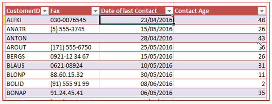
Objective: Identify Customers whose Date of Last Contact > 28 days ago using Conditional formatting.
Step1: Develop a formula and test it copies correctly
Note the use of a Mixed Address ($C11) which is referring to the Date of Last Contact

Step 2: Copy the formula into the New Formatting Rule for just one cell. Format as required.
Step 3: Use the Format painter to copy that formatting and apply it to all cells in your list.

Step 4: Check the Conditional Formatting Rules Manager for any accidents.
Step5: Re-apply any numeric formatting as necessary.


Payments processed by

